过去几周发生了很多事情。我相信现在大家最关注的一定是 OpenAI 的 GPT-6 Astra。尤其是关于它的性能表现、循环 Transformer/循环深度方面的特性，以及有关 Astra 在“隐藏”其推理轨迹（即思维链）的传闻。

因此，在这篇文章中，我想先谈谈对 Astra 的一些简要印象，以及我对这一切未来走向的一些思考。然后，我会详细讨论什么是“循环 Transformer”，以及它如何（或者更确切地说，是否）与隐藏思维链有关。

最后，在介绍完循环 Transformer 的基础知识之后，我想重点分享一些近期关于该主题的研究论文所带来的新见解。

1. GPT-6 Astra 初步印象

先说重点。在深入架构传闻及相关研究文献之前，让我先简要总结一些关于 GPT-6 Astra 的观察和零散信息。

上周，OpenAI 的新模型 GPT-6 Astra 高调发布。过去几天我一直在使用它，这是一个极其出色的模型，很可能是我写这篇文章时用过的最好模型。但具体来说，它到底改进了什么，又是如何改进的？

1.1 Astra 基准测试

Astra 是我目前用过最好的模型，而且在 3D 渲染和动画任务上（相对于其他模型）表现得格外突出。我的意思是，虽然它在几乎所有类别（写作、数学、编程等）上都超越了其前代 GPT-5.6，但在图形演示方面尤其如此。

我们也能在基准测试中看到这一点。例如，如下所示，GPT-6 Astra 在数学和编程方面非常出色。

其中一个亮点（未在图中显示）是 Astra 在 ARC-AGI-3 基准测试 上也达到了 99.9%（GPT-5.6 Sol 仅为 7.8%），该测试衡量的是逻辑谜题求解与泛化能力的综合表现。不过，数学、编程和计算机使用相关的基准测试更有意思，因为它们更接近实际应用场景。

回到 Artificial Analysis Coding Agent Index v1.4（上图右下角），该指数综合了多项智能体编程任务，GPT-6 Astra 显然处于前沿，但并未拉开巨大差距。这一点也可以从下面展示的综合 Artificial Analysis Intelligence Index 中看出，该指数综合了不同类型的任务，而不仅仅是编程任务。

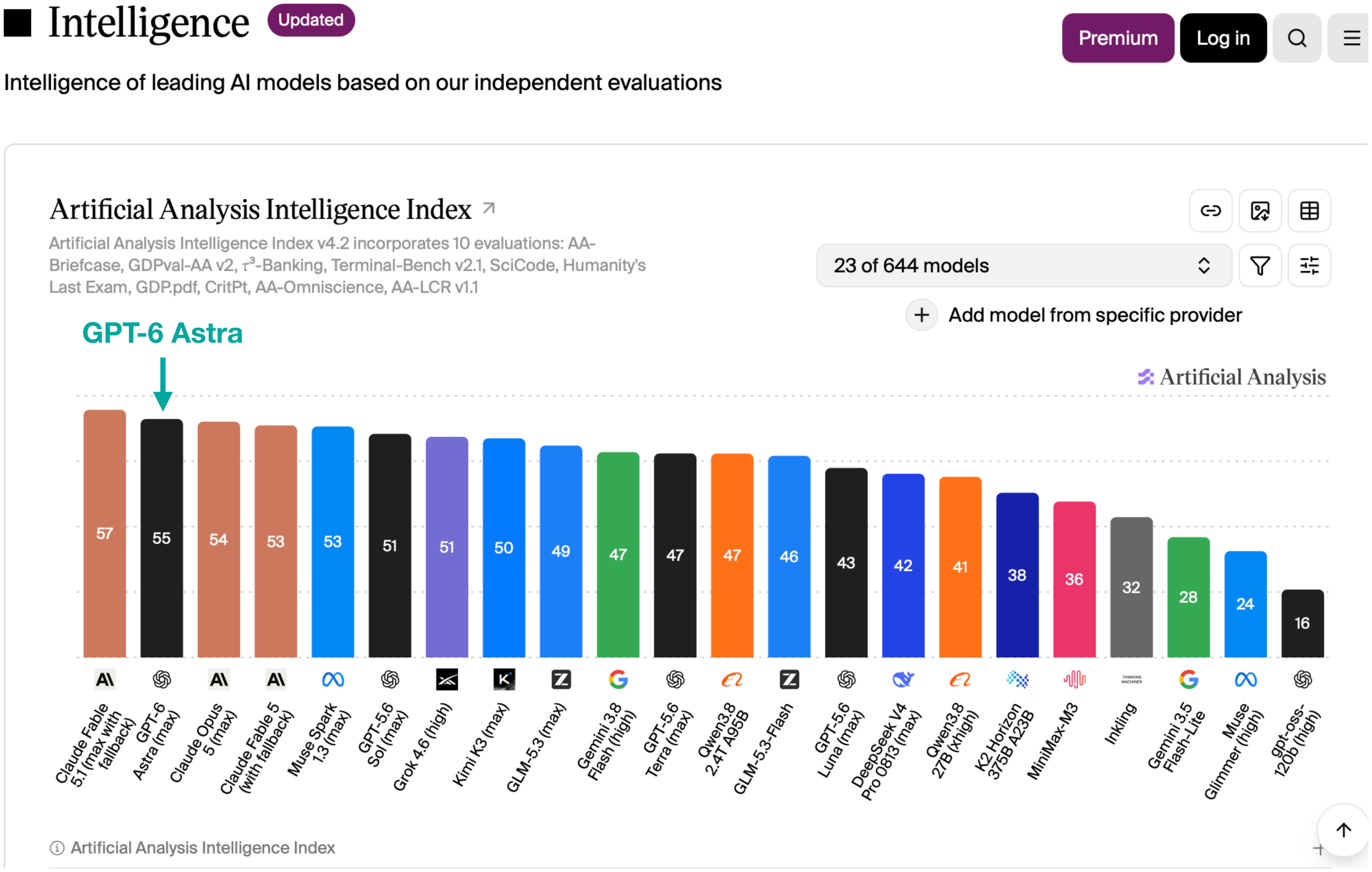
现在，Artificial Analysis 基准测试的一大优势在于它们是独立进行的，因此可能比模型开发者自行评估的基准测试更值得信赖。

测试框架的搭建取决于具体基准。例如，GDPval-AA 和 AA-Briefcase 在它们所比较的不同 LLM 上使用了开源、极简的 Stirrup 测试框架。在上述 Intelligence Index v4.2 中，Terminal-Bench v2.1 使用 Terminus 2，而 τ³-Banking 使用 τ-Bench 测试框架。另外，Coding Agent Index 也对比了不同的编程智能体测试框架。

对于使用共享测试框架的评估而言，这使其更像是同类之间的直接对比。与此同时，在模型训练期间，模型通常主要针对某一个核心测试框架进行开发（而在其他测试框架上的微调较少）。此外，这个核心测试框架往往是为了适配并放大模型的优势而开发的。

因此，某些智能体评估可能低估了 Astra 在其核心测试框架中的实际表现。这一因素对其 Intelligence Index 得分的影响程度，需要通过在同一任务上跨不同测试框架对比 Astra 来加以验证。

顺便提一句，正如一位同事最近向我建议的那样（Claude Code 的负责人也给出了同样的建议），删除（或归档）你现有的一些 AGENTS.md 内容和 SKILL.md 文件或许不失为一个好主意，因为更新的 LLM 在理解提示词和解决当前问题方面已经变得更加高效。过多的手把手引导反而可能不必要地束缚新模型，导致解决方案质量下降。

当然，我并不是建议再也不使用 SKILL.md 文件，但在某些工作流程中，由于模型无需重新摸索这些内容，复用它们确实能提升效率。不过我想说的是，有些工作流程根本无需描述，而且“旧”的描述可能已不再理想，大语言模型或许能想出更好的解决方案。因此，也许是时候更新或重新生成这些指令文件了。

1.2 计算机使用能力

GPT-6 Astra 在图像和渲染任务上似乎异常强大。当这些任务涉及与图形用户界面交互时，它也展现出计算机使用能力，也就是说，该模型能通过 Codex/ChatGPT 应用在你本地计算机上操作软件。

计算机使用是模型相较其他产品真正出彩的地方，而任何与图形相关的操作也都能在社交媒体平台上构成有趣且直观的演示。网上有大量令人印象深刻的演示案例，从 在 Blender 中渲染纽约市 到 虚拟开放看房导览，不一而足。

举一个例子，下面是一组对比，我让 GPT-6 Astra Medium 和 High 在我电脑上使用鼠标，在 浏览器版 MS Paint 中重新绘制一张我的照片（没有用 Extra High 和 Max，因为我不想浪费我所有的 token :))。

这不仅凸显了模型的艺术能力，更重要的是，它展示了模型在用户计算机上使用工具的能力（本例中即 Paint；你可以看到模型通过鼠标光标操作界面）。

这并不是第一个在工具框架（harness）内具备通用计算机操作能力的模型。例如，自今年早些时候起，我就成功使用 GPT 模型完成了一些 UI 任务（例如 Excel 中与费用相关的任务）等。然而，计算机操作是一项相对较新的能力，由工具框架赋予，而且通常感觉还不够成熟。这也在情理之中。LLM 是文本模型，因此自然而然地，最容易出成果的方向是写作、编程以及使用 API 和 CLI。

与此同时，有许多工具和软件（目前）并未提供 CLI 接口，与其等待有人设计出那样的接口，为什么不改进模型，让它们能够使用图形用户界面呢（而且如前所述，这无论如何都能带来漂亮且令人印象深刻的演示效果）？这在某种程度上类似于正在兴起的人形机器人研发。诚然，人形机器人并非最高效的机器人，例如在流水线上，那里已有专用机器。但它们用途广泛。

因此，我预计未来几个月（或几年）也将是 LLM 和智能体工具框架层面计算机操作能力不断精进的时代。也就是说，除了现有能力之外，在扩展数学和编程能力的同时，模型在训练中也会越来越多地考虑到计算机操作。而这也会让 LLM 在科技领域之外的日常计算机任务中更容易被使用（“嘿，ChatGPT，请帮我报税” ：））

1.3 计算机操作训练

计算机使用这一趋势也与 近期的报道 一致，即 OpenAI 购买了数万台 Mac Mini 和 Mac Studio 用于强化学习。因此，这里的 Mac 并不是真正用来训练模型（这方面用 GPU 更好），而是在模型训练过程中让模型接触 macOS，使其学会使用该操作系统及其中的工具。

那么，在上述 Mac 上进行计算机使用训练是如何运作的呢？简而言之，这些 Mac（更准确地说，是它们的 macOS 操作系统）充当了模型在训练期间可以与之交互的环境。

基本工作流程如下：

1. 通过给模型一个任务来提示它，例如“打开应用 xyz 并执行 abc”。

2. 向模型提供 macOS 界面的截图（这通常由测试框架完成）。

3. 然后大语言模型预测鼠标/键盘操作（点击、按键、滚动等）。

4. 在 Mac 上执行这些操作（同样，这由测试框架完成）。

5. 在执行上一步的操作后，将更新后环境的新截图反馈给模型。

6. 重复步骤 2-5，直到任务成功或失败。

7. 使用成功/失败信号和验证器（或评分器）作为训练反馈，包括在后训练阶段进行强化学习；这与常规的带可验证奖励的强化学习（RLVR）类似。

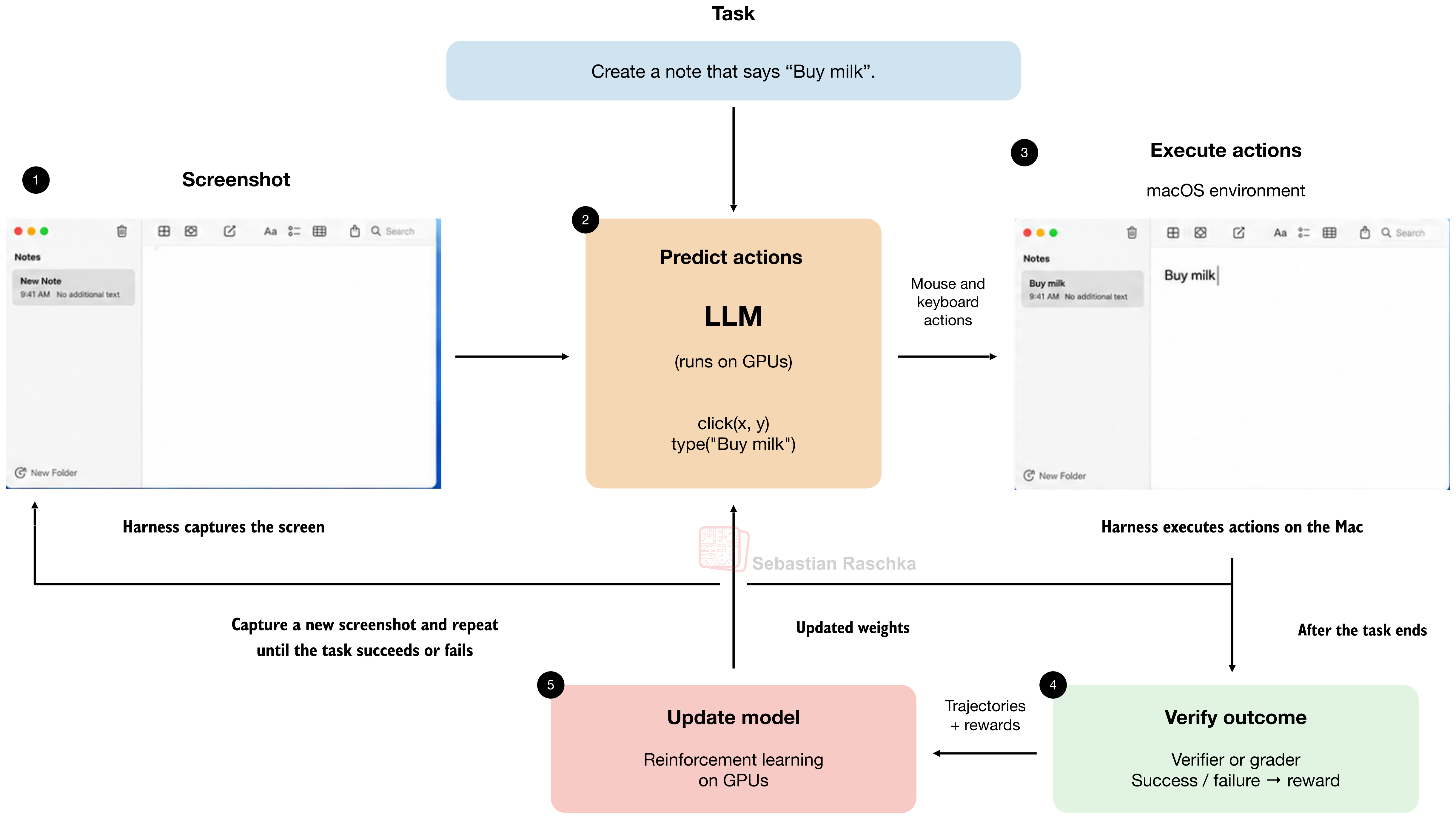
再次强调，Mac 在这里主要充当环境角色，而不是训练期间运行或更新模型的机器。模型很可能运行在 NVIDIA GPU 上，并通过 API 馈送给上述 Mac。顺便提一下，NVIDIA 的 CEO 提到，GPT-6 Astra 正在约 10 万块 Grace Blackwell GPU 上进行训练。

1.4 GPT-6 Astra 仍然是一个推理模型

上一节讨论的计算机使用训练重点，并非训练流程中的根本性范式转变。GPT-6 Astra（以及可预见未来中的任何大语言模型）仍然是一个推理模型。这意味着该大语言模型通过带可验证奖励的强化学习（RLVR）进行训练，并产生中间推理轨迹（思维链）。

但我将在本文稍后部分讨论 GPT-6 Astra 的推理模型特性（尤其是关于隐藏思维链的方面）。

2. 循环 Transformer

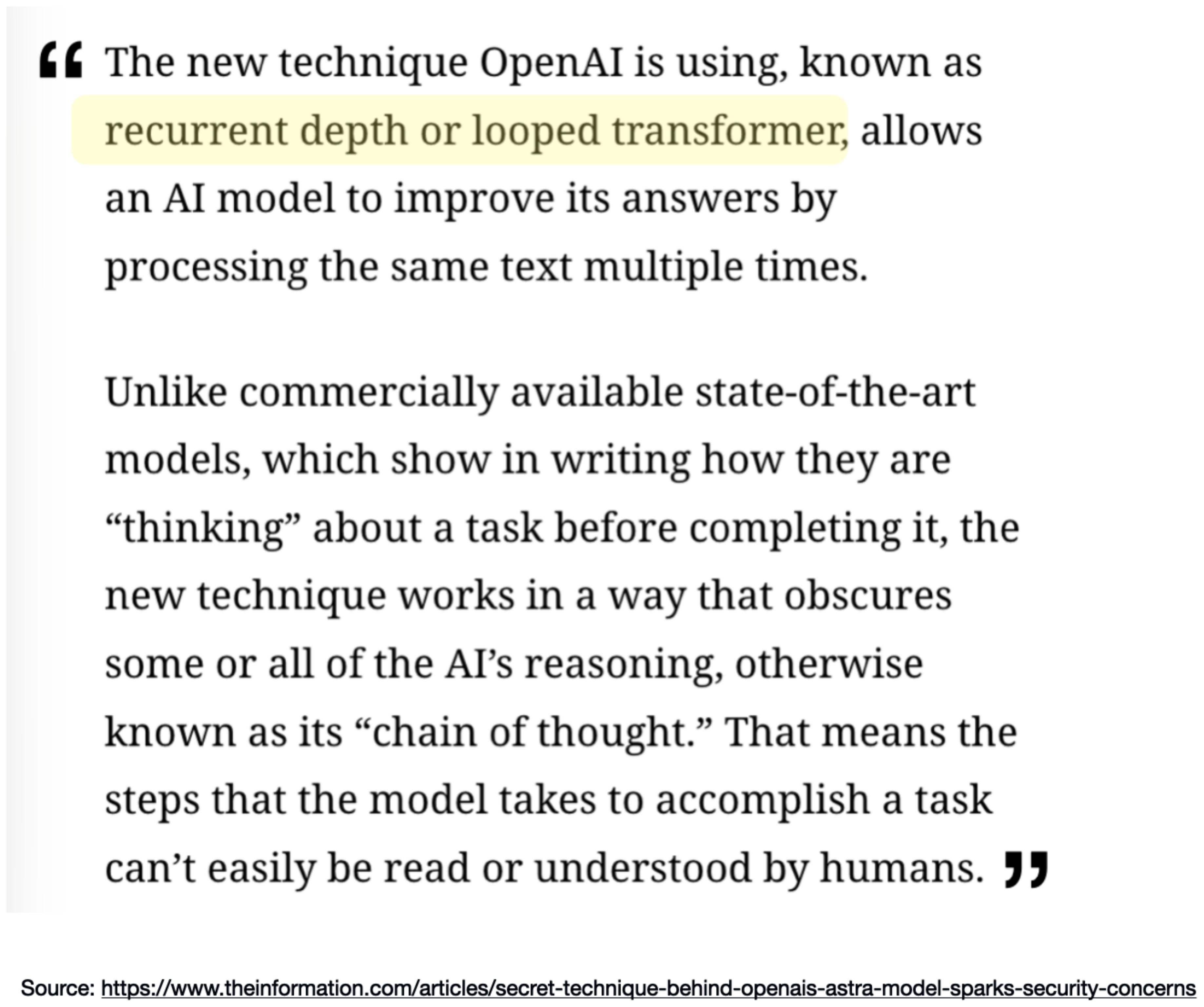
话虽如此，在官方模型发布前两天左右，新闻杂志 The Information 发布了一篇文章，报道称根据一些内部消息，Astra 采用了一种名为“循环深度”或“循环 Transformer”的概念。

由于大语言模型架构属于我的专业领域，也是我的热情所在，我制作了一个简短的讲解视频，解释一般的循环 Transformer 机制，并回应了关于隐藏推理链的评论，你可以在下方找到该视频。

在接下来的小节中，我会先解释什么是循环 Transformer，并在本文后面重新讨论关于隐藏思维链的评论。

（循环 Transformer 的解释可能看起来有点长，但我真的认为这有助于建立对该技术的基础理解，而这对于判断“它掩盖了推理痕迹或思维链”这一说法是否成立很有用。）

2.1 复用 Transformer 模块

那么，什么是循环 Transformer？

循环 Transformer 本质上是一种架构上的微调，其核心思想是将中间表示多次（而非仅一次）通过相同的 Transformer 模块。与单纯增加更多模块相比，这里的“诀窍”在于这些多次传递过程中权重保持不变。

定义与术语

在本文中，我将使用以下术语：

• 一个 Transformer 模块 是包含注意力机制、前馈模块、归一化和捷径连接的一个单元。这些模块在论文中通常被称为“Transformer 层”。

• 一个 堆栈 是一系列 Transformer 模块的序列。

• 一次 模块应用 意味着将输入通过一个 Transformer 模块运行一次。

循环 Transformer 并非新事物，其基本思想早在 2018 年的 Universal Transformers 论文中就已出现。但在讨论 Universal Transformer 之前，让我们先从一个更简单的例子开始：Nanbeige4.2-3B，这是一个最近发布的开源权重 LLM，于 7 月推出，我今年夏初曾在 Substack Notes 和我的 LLM 架构画廊 中介绍过它。

Nanbeige 架构如下图所示，本质上看起来就像一个常规的 Transformer。不过请注意，它多了一条（橙色的）箭头，循环回到 Transformer 堆栈的开头。

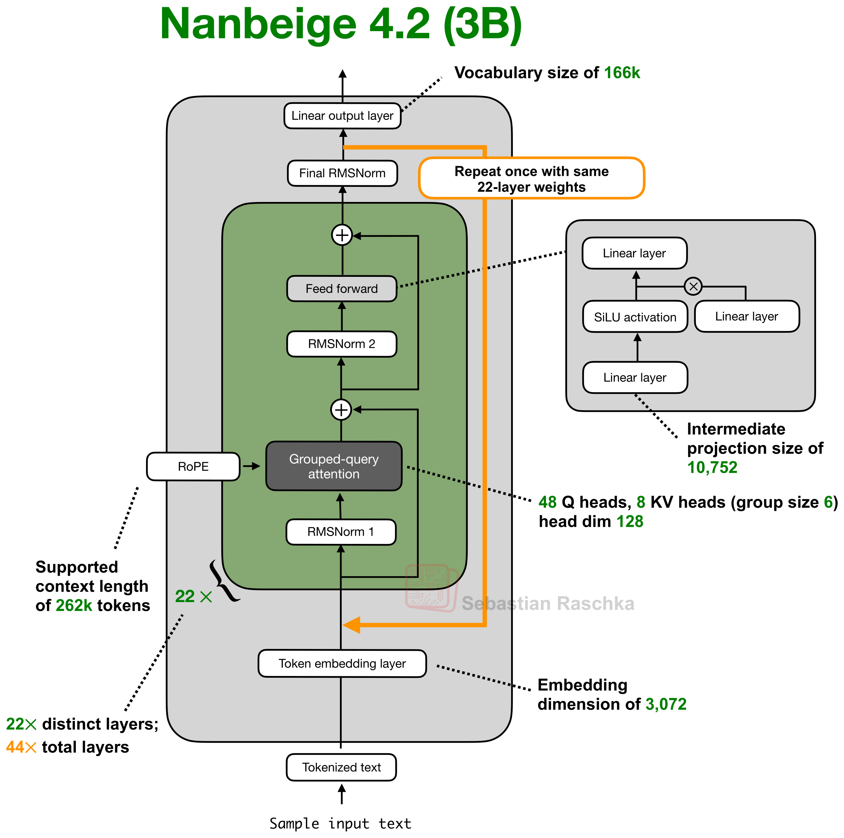
让我们从下往上梳理这个过程。首先，与任何其他基于 Transformer 的大语言模型一样，输入文本会被分词并转换为嵌入向量。随后，这些向量依次通过 22 个 Transformer 块，而这 22 个块中的每一个都有各自的权重。

不过，这里的循环 Transformer 之处在于：第一次通过之后，隐藏状态会被重新送入这相同的 22 个块。也就是说，块 1 再次被应用，接着是块 2，依此类推直到块 22。

如果我们把这个计算过程展开来看，就会有 44 次 Transformer 块的应用。然而，与拥有 44 个不同块的常规 Transformer 相比，第二组 22 次块应用复用了第一组的权重。例如，第 23 次块应用使用块 1 的权重，第 24 次块应用使用块 2 的权重，依此类推。

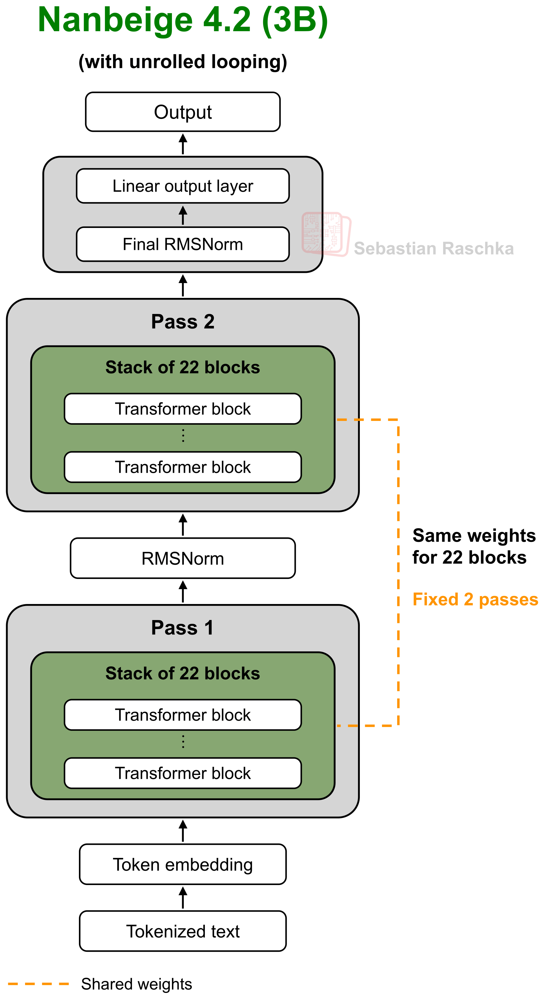
所以，这里的整体思路是：我们无需增加另一套 Transformer 权重，就能将有效深度从 22 次块应用提升到 44 次。

顺便问一下，为什么是 2 轮而不是 3 轮、4 轮或更多？Nanbeige 论文中细节不多，但他们表示这基本上是最高效的配置。把循环从 2 轮增加到 3 轮可以提升建模性能，但额外的计算成本并不划算。

2.2 循环成本

那么，我们为什么要普遍采用这种循环方式呢？这本质上是一种替代方案，用来替代通过增加更多 Transformer 层来把模型做得更大的做法。

例如，一个使用 22 个 Transformer 层循环两次的模型，其（Transformer 层）参数量大约是拥有 44 个传统层模型的一半。

这样就能减少存储权重所需的内存。顺便提一句，嵌入层和输出层通常规模较大，在总参数量中占相当大比例，但它们不在此对比范围内。（以 Nanbeige 4.2 3B 为例，嵌入层和输出层约占 3B 总参数量的 25%；如果在这两层之间共享权重，我们可以将其降至 12.5%。）

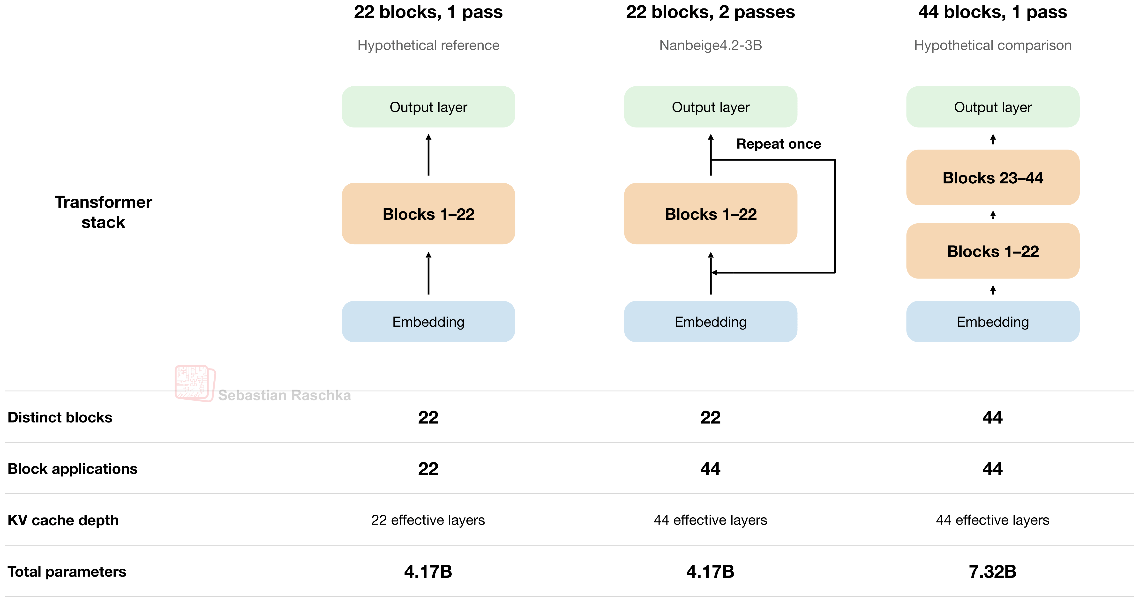
当然，在循环中复用相同的模块仍然需要计算。更准确地说，在前向传播过程中，我们需要将中间输入依次通过 44 次模块应用。而在训练时，梯度会反向流过共享模块堆叠的两次重复。因此，与仅使用一次这 22 个模块相比，这会增加大量计算量。实际上，其开销与使用 44 个独立模块相当（区别仅在于优化器需要更新的独立参数更少；反向传播仍然要跑完全部 44 次模块应用）。

此外还有 KV cache，它存储之前 token 的注意力键和值，以便在传统 Transformer 和循环 Transformer 的每一步下一个 token 生成中复用。顺便提一下，如果需要，我有一篇关于 KV 缓存的独立文章：

但回到正题。尽管循环 Transformer 中存在权重共享，但第二次通过时进入模块的中间状态是不同的。因此，在 KV 缓存中，这两组 Transformer 堆叠所产生的键和值也会不同（就像无循环的情况一样）。所以，在 KV 缓存方面也没有任何节省。

为了更具体地说明，例如，考虑第 1 次和第 23 次模块应用，在循环 Transformer 设置中它们都使用模块 1。但每次应用仍然需要自己的 KV 缓存条目。因此，由于我们必须为两次通过分别保留缓存，这 22 个模块的重复堆叠与具有 44 个独立模块的传统 Transformer 具有相同的 KV 缓存需求。

有趣的是，Nanbeige 的研究人员在论文中报告称，他们尝试了在不同轮次之间共享 KV cache。这自然将 KV cache 大小减半，但模型性能不如使用独立 cache 的版本（也就是他们最终发布的版本）。

在继续讨论其他循环 Transformer 设计之前，先把 Nanbeige 这部分讲完——他们的技术报告还讨论了另外两个选择或权衡。

1. 从头训练这种循环架构，效果优于通过 upcycling 方式改造一个已经预训练好的 Transformer。

2. 如前一小节所述，两轮循环是他们在权衡后偏好的选择。更多轮次只带来微小的额外收益，同时会拖慢训练速度，并让优化过程变得不那么稳定。

所以，循环轮数是我们必须做出的另一个架构选择。如前所述，在 Nanbeige 中，这个数字固定为二。但我们也可以让它根据 token 而变化，接下来我们就会看到这一点。

2.3 通用 Transformer 与灵活的循环次数

现在，让我们回到Universal Transformers。在 Nanbeige 中，我们将 22 层 Transformer 块堆叠后应用两次。而在 2018 年的 Universal Transformer 论文中，他们反复应用同一个 Transformer 块，而不是重复应用一整个 Transformer 块堆叠。不过，核心思想是相似的。

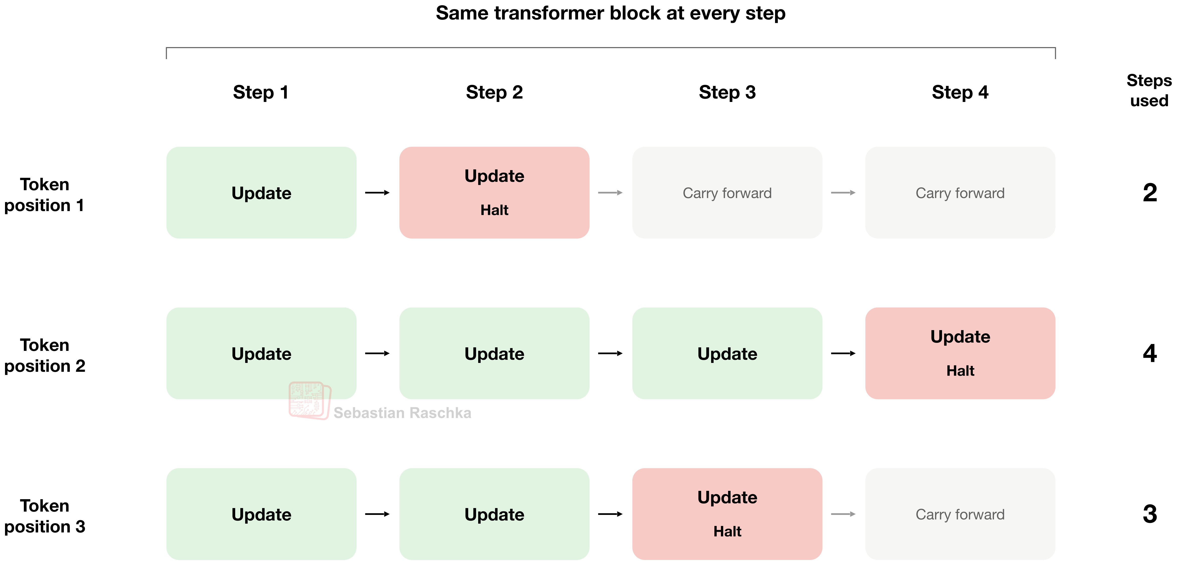
此外，步数可以是固定的，但论文也探讨了自适应停止机制。例如，某个特定位置的 token 可能只经过一到两次循环，而另一个 token 可能经过三到四次循环，以此类推。这赋予了模型灵活性，可以将算力分配给那些能从额外计算中受益的 token。

循环次数是如何决定的呢？这里，模型使用一个小型的、经过训练的函数，在每一步为每个位置输出一个所谓的停止概率。模型将这些概率在连续的循环中累加，一旦总和超过某个阈值，便停止在该位置的循环。此外，最大循环次数也限制了计算量，以防万一。

另一个循环 Transformer 的例子是字节跳动的 Ouro，我也在我的 LLM 架构画廊 中介绍过它。例如，Ouro-Thinking 2.6B 将相同的 48 个 Transformer 块堆叠应用了四次。这意味着进行了 192 次块应用，同时只为 48 个不同的块存储权重。基本上，这比 Nanbeige 的情况更为极端。此外，一个学习得到的出口门控为不同的出口分配概率，并且对累积概率设置一个阈值，以决定哪一次传递提供输出。因此，它也借鉴了 Universal Transformer 的自适应停止思想，而 Nanbeige 并未采用这一点。（不过，这里有一个实际的注意事项。已发布的 Hugging Face 实现 会在选择输出之前计算所有配置的传递次数，因此循环次数实际上似乎是硬编码为 4 次）。

2.4 路由灵活循环次数

另一种方法是 Mixture-of-Recursions，这是 2025 年的一篇论文，本质上是对前面讨论过的 Universal Transformer 的一种更精妙的改进版本。与 Universal Transformer 类似，每个 token 会一次或多次通过 Transformer 模块，如下图所示。然而，其创新之处在于如何针对每个 token 单独确定这个循环次数。

在论文的下面这张图中，被循环（重复）的堆叠层在这里被称为递归块。它包含多个 Transformer 模块，并位于独立的第一个和最后一个 Transformer 模块（标记为 Layer 0 和 Layer L-1）之间。

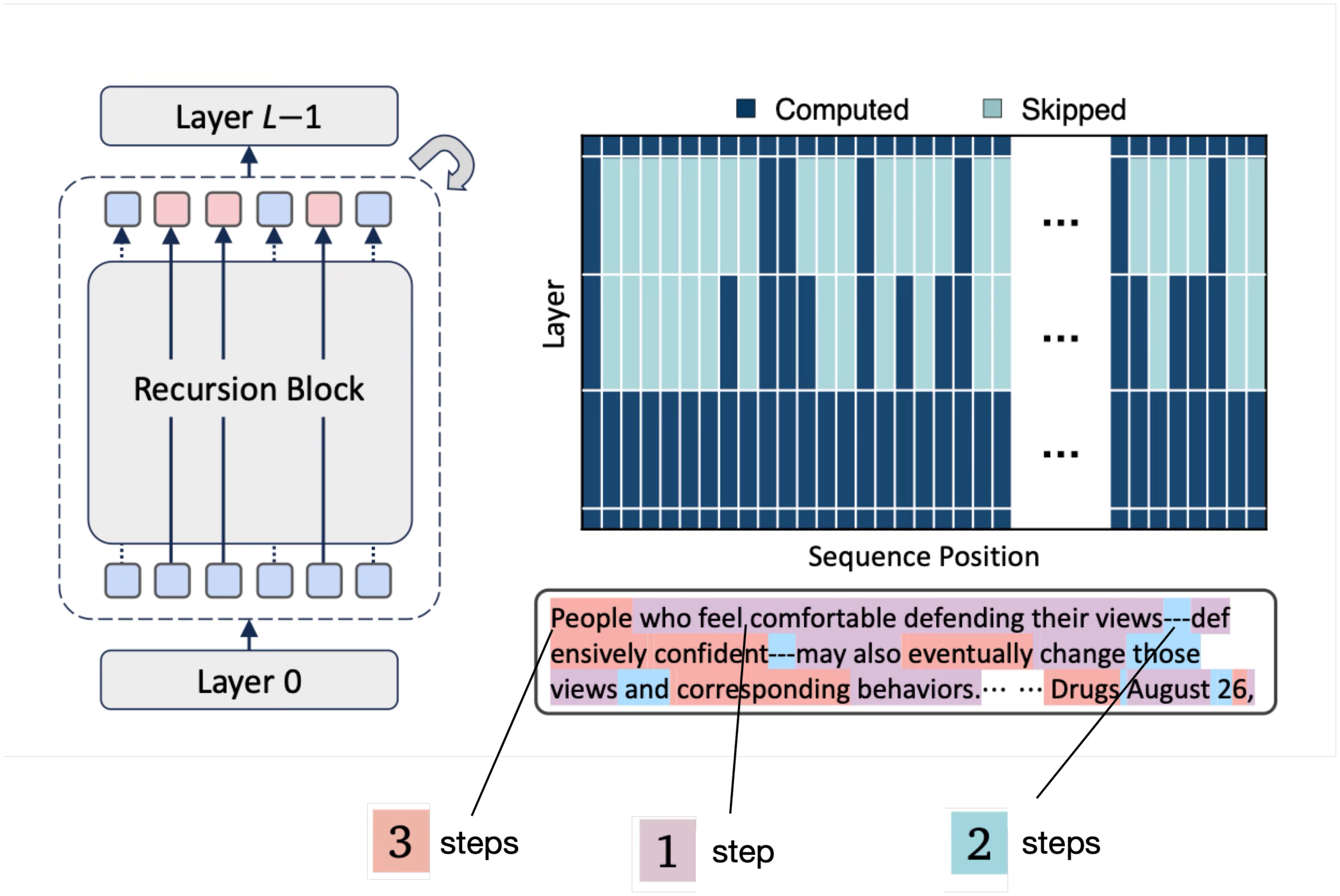
模型如何决定一个 token 应该通过递归块多少次？在前面讨论的 Universal Transformer 中，这是基于每一步学习到的停止概率来决定的。而这里的 Mixture-of-Recursion 方法则使用一个小型的、经过学习的路由器。这与混合专家模型中的路由思想类似，区别在于这里的路由决策决定了应用共享堆叠层的次数。

路由器作用于 token 的隐藏表示，而隐藏表示中也包含该 token 的上下文信息。因此，我们不应将其理解为：某个特定 token 的每次出现都被分配相同的递归次数（例如，上图中的单词“People”并不总是经过 3 次循环）。这个决策会根据该词出现的位置以及其前面的内容而改变。

那么，路由具体是如何工作的呢？论文探讨了两种做出这种路由决策的方式，如下图所示。

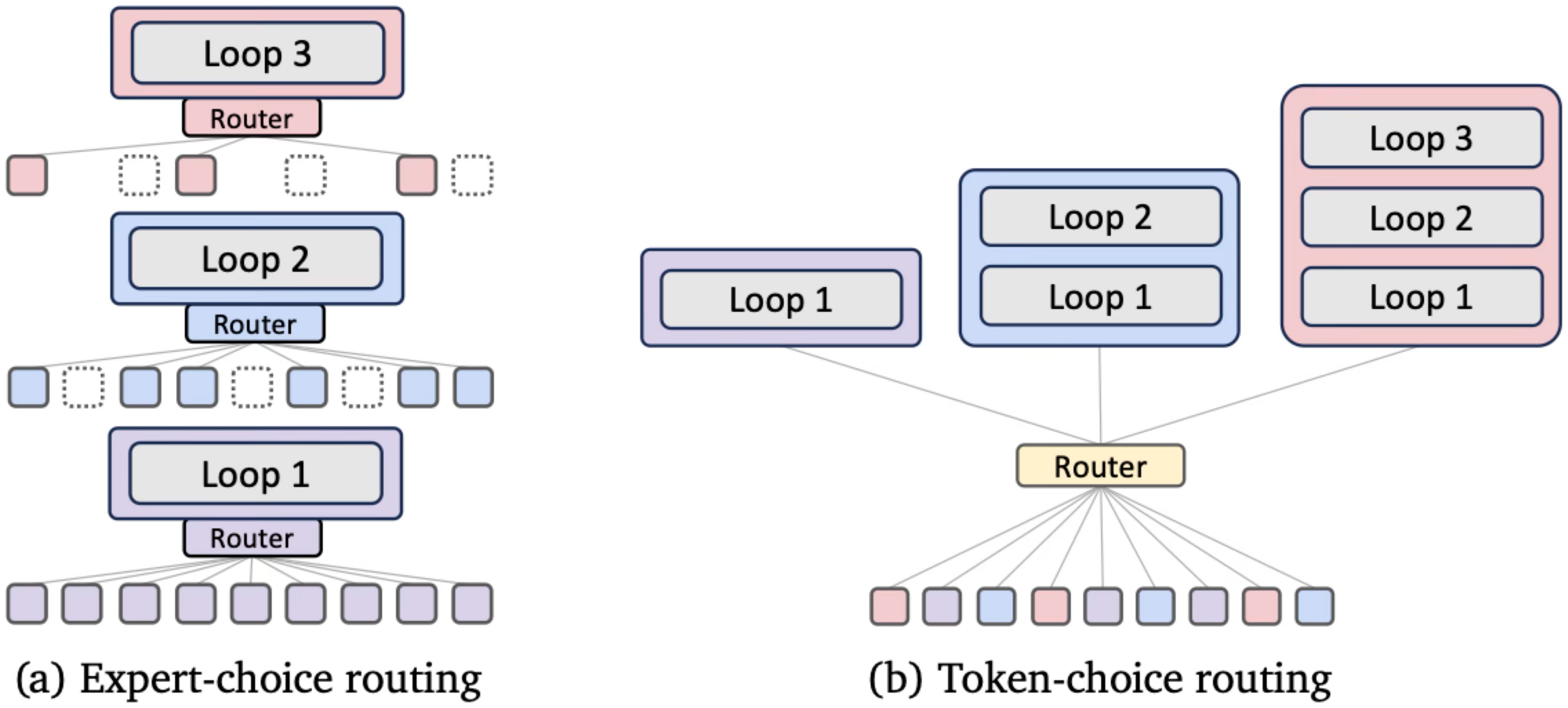
在上图左侧子图中展示的 专家选择路由（expert-choice routing）中，每个递归步骤会选择它将处理哪些 token。退出的 token 将从后续步骤中被排除。在右侧展示的 token 选择路由（token-choice routing）中，路由器在开始时做出一次决策，将每个 token 分配到具有一次、两次或三次递归的路径上。

在两种情况下，Transformer 的权重都会在多次递归中被复用，这与 Nanbeige 等模型类似。但额外的灵活性来自于选择每个 token 获得多少计算量。模型及其路由器是一起训练的，因此模型在训练过程中会学会如何与这些不同的路径配合工作。

2.5 这种方法效果如何？

下面这篇 Mixture-of-Recursions 论文中的图表，比较了不同模型规模和计算预算（x 轴）下，普通 Transformer（Vanilla）、固定递归 Transformer（Recursive）以及 Mixture-of-Recursions（MoR）的表现。

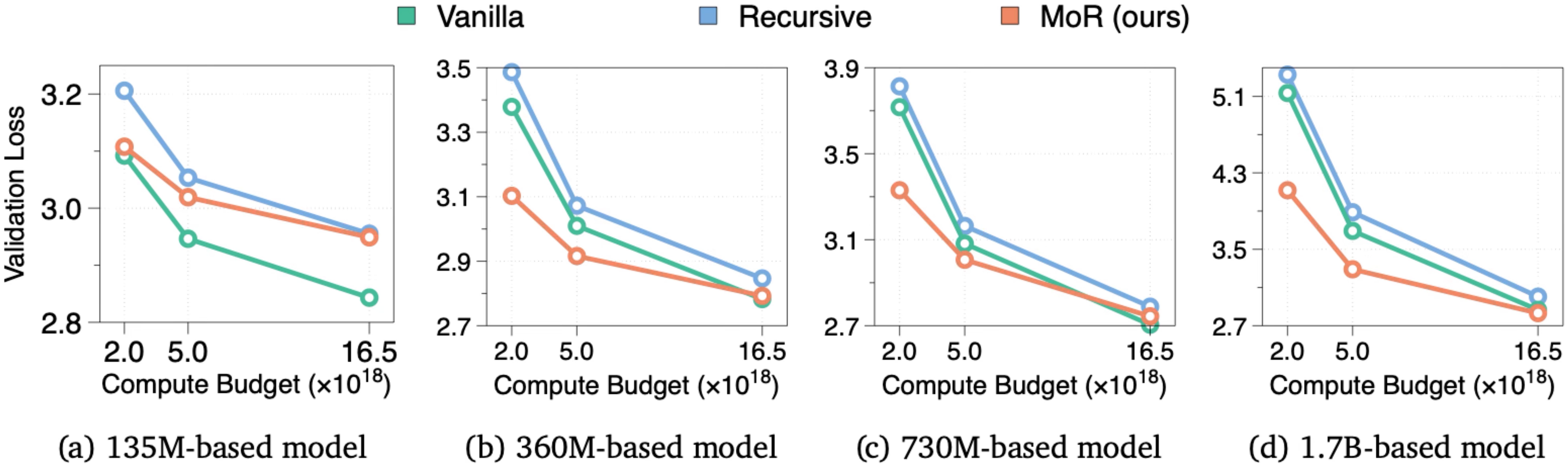
在最小的模型规模下，普通 Transformer 表现最佳。对于较大的模型，Mixture-of-Recursions 迎头赶上，并且通常表现更好，尤其是在较小的训练预算下。在最大的预算下，几条曲线非常接近。因此，优势取决于模型规模以及我们在训练上投入的计算量。

这里的另一个细节是，相同的训练计算量并不一定意味着相同数量的训练 token。通过跳过部分计算，Mixture-of-Recursions 可以在相同的预算内处理更多的 token。

我认为这是一个有趣的例子，因为它表明在循环 Transformer 这一思路中存在多种选择，即每个位置有多少个循环，以及如何决定这一点。

所以，简而言之，我们可以说，在固定计算预算下，如果模型足够大，使用循环 Transformer 可以提高模型质量。（这也说明了进行大规模实验的重要性；例如，如果只看较小的 135M 参数模型，我们可能会得出相反的结论。）

3. 附注：循环神经网络（RNN）

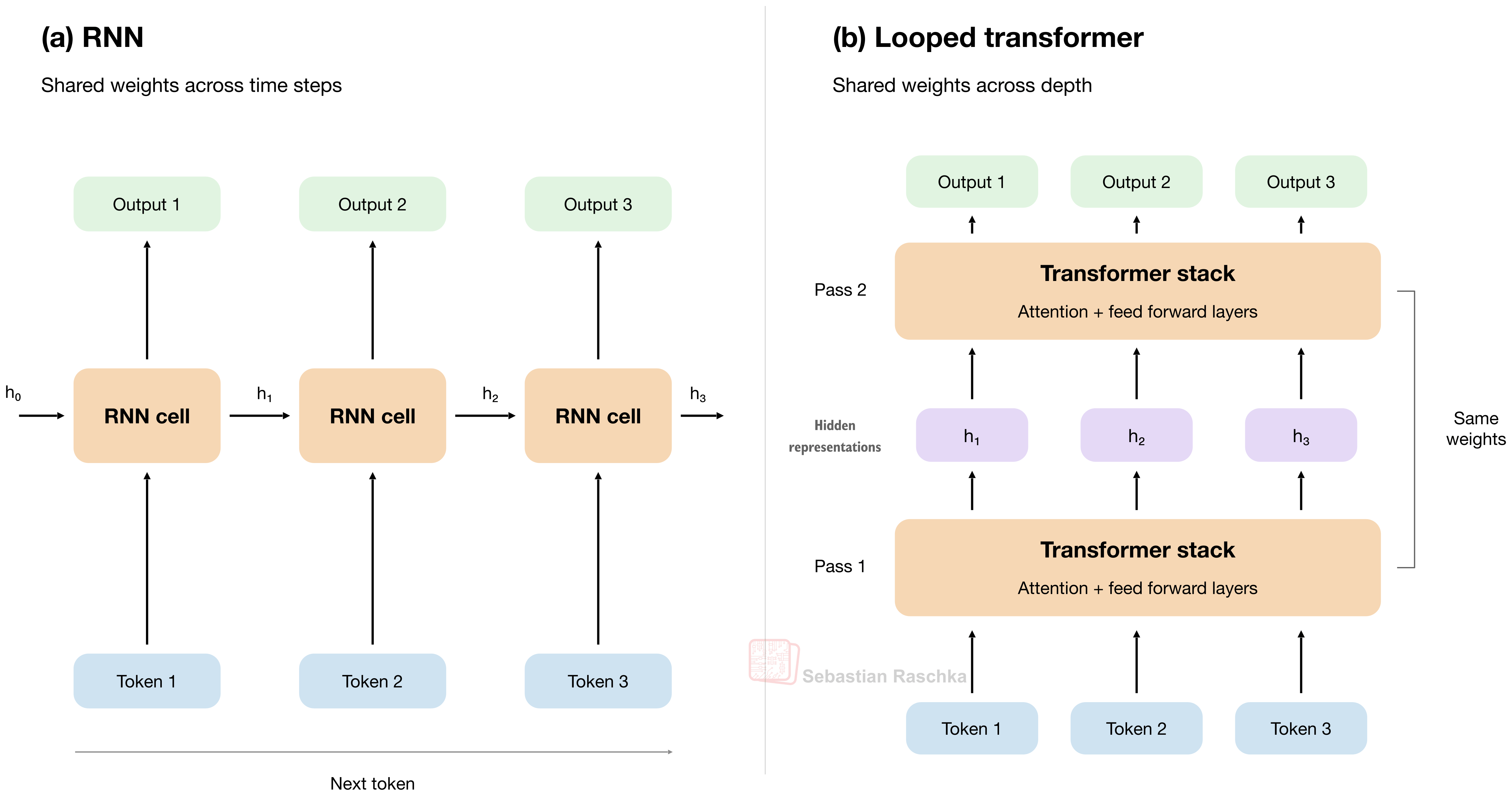
顺便说一句，如果你有深度学习（甚至 1990 年代的人工神经网络）背景，这种循环或“循环深度”的概念应该会让你感到有些熟悉。还记得循环神经网络（RNN）吗？RNN 的核心思想就是复用上一次迭代的层（权重）。

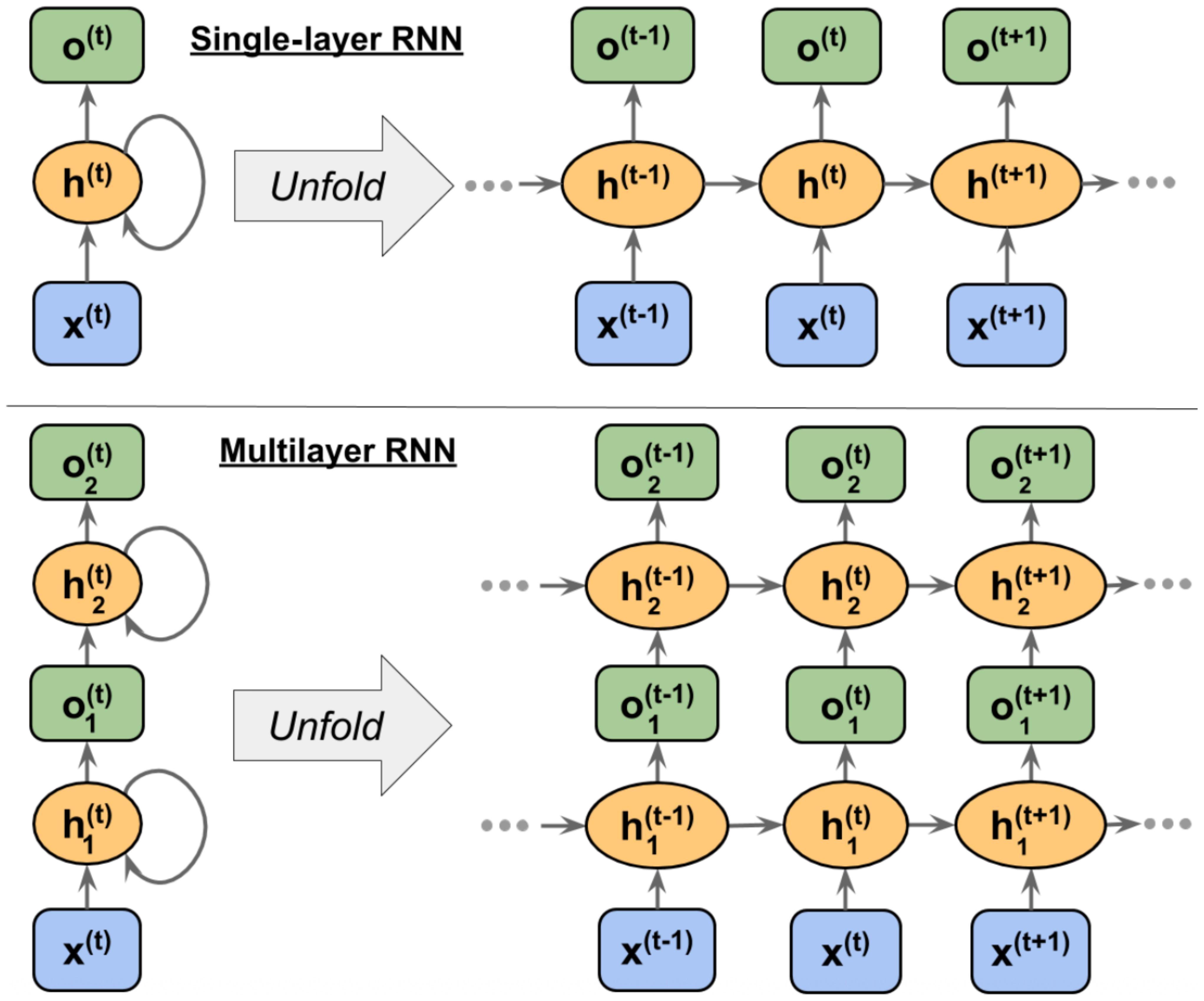
主要区别在于，RNN 是在时间步之间复用权重。也就是说，隐藏状态会从一个 token 传递到下一个 token。而在循环 Transformer 中，token 的循环是跨越架构深度的。

或者换句话说，在传统的 RNN 中，每一步都接收输入序列中的下一个元素以及上一步的隐藏状态。因此，当 RNN 在处理一段文本时，它一次读取一个词或 token，并将前面词的信息通过隐藏状态向前传递。

在循环 Transformer 中，给定 token 的中间表示会多次经过 Transformer 堆叠层。模型仍然使用注意力机制在 token 之间传递信息。

如果这个类比让你觉得有点困惑，也不用太担心。也许一个更简单的理解循环 Transformer 的方式是：把它们看作是对 Transformer 块的复用，类似于把模型做得更大，但采用了权重共享。

4. Astra 真的使用了循环 Transformer 架构吗？

在我们讨论循环 Transformer 机制是否像前面 The Information 引述的传闻那样掩盖了推理轨迹之前，GPT-6 Astra 到底有没有使用循环 Transformer 的概念？

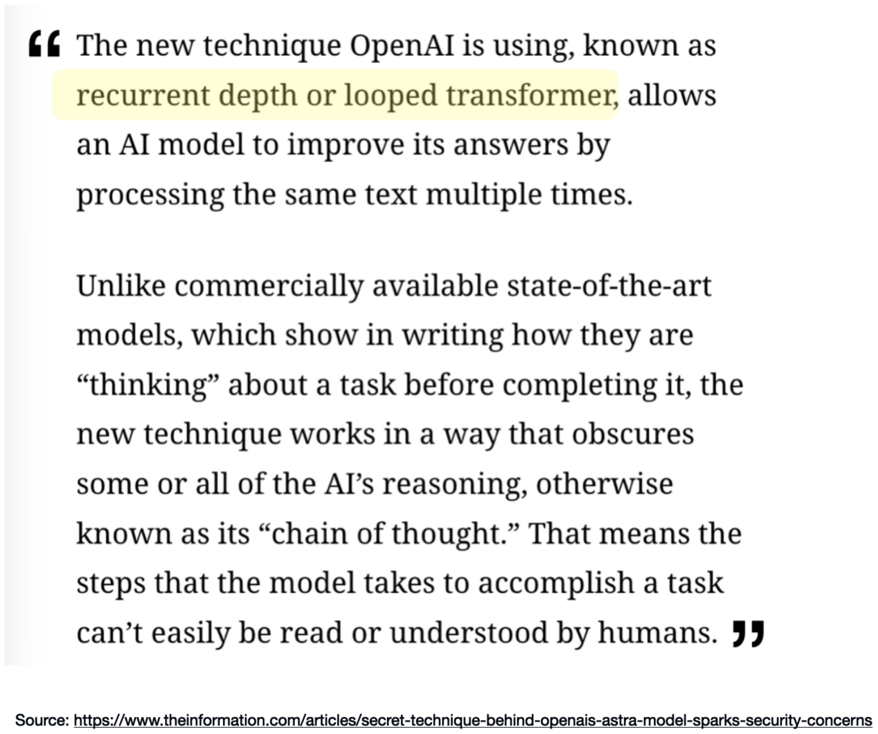
我们要记住，这仍然只是传闻或独家爆料，尚未得到官方证实。如果这个模型是开放权重的，我们当然可以自己核实，但就目前而言，我们只能依赖未经证实的报道。

不过，我认为 GPT-6 Astra 极有可能采用了循环 Transformer 的某些方面。首先，有上述报道作为依据。其次，这项技术在过往研究中已展现出潜力（如前文所述），那何乐而不为呢？第三，OpenAI 首席科学家说过下面这段话。

[...] 我们当前前沿模型（包括 Astra）的计算图深度，与 GPT-4 相比在 2 倍以内。[...]

然而，这并不能明确证实循环 Transformer 架构，也可能只是意味着他们使用了数量翻倍的常规 Transformer 块。

在我看来，Astra 之所以成功（即建模性能出色），很可能主要归功于其他原因，也就是改进的训练配方和训练数据。

循环 Transformer 的调整或许能带来一点帮助，但我认为 The Information 高估了它的贡献。

5. 隐藏思维链

接下来，我们终于要直面这个房间里的大象：循环 Transformer 是否真的会模糊推理痕迹？

首先，OpenAI 从一开始就在向用户隐藏（大部分）推理痕迹，至少从 OpenAI o1 开始就是如此。所以，对于终端用户来说，应该不会有太大差别。

因此，关于可解释性的担忧主要针对的是模型开发者。

无论如何，我认为循环 Transformer 并不是隐藏或模糊思维链的重要推手。为了解释我自己的推理（无意双关），让我们退一步，先说明推理模型的工作原理。

5.1 推理简述

推理模型通常会在生成最终答案之前先产生中间步骤。这些步骤使用常规文本 token（在某些用户界面中可选择对用户隐藏），被称为推理痕迹或思维链。

例如，假设我们要求两个数，它们的和为 10，积为 21。在下图中，模型起初尝试 5 和 5。虽然和是正确的，但积是 25，而不是 21。接着，它又尝试 3 和 7，并再次检查这两个条件。

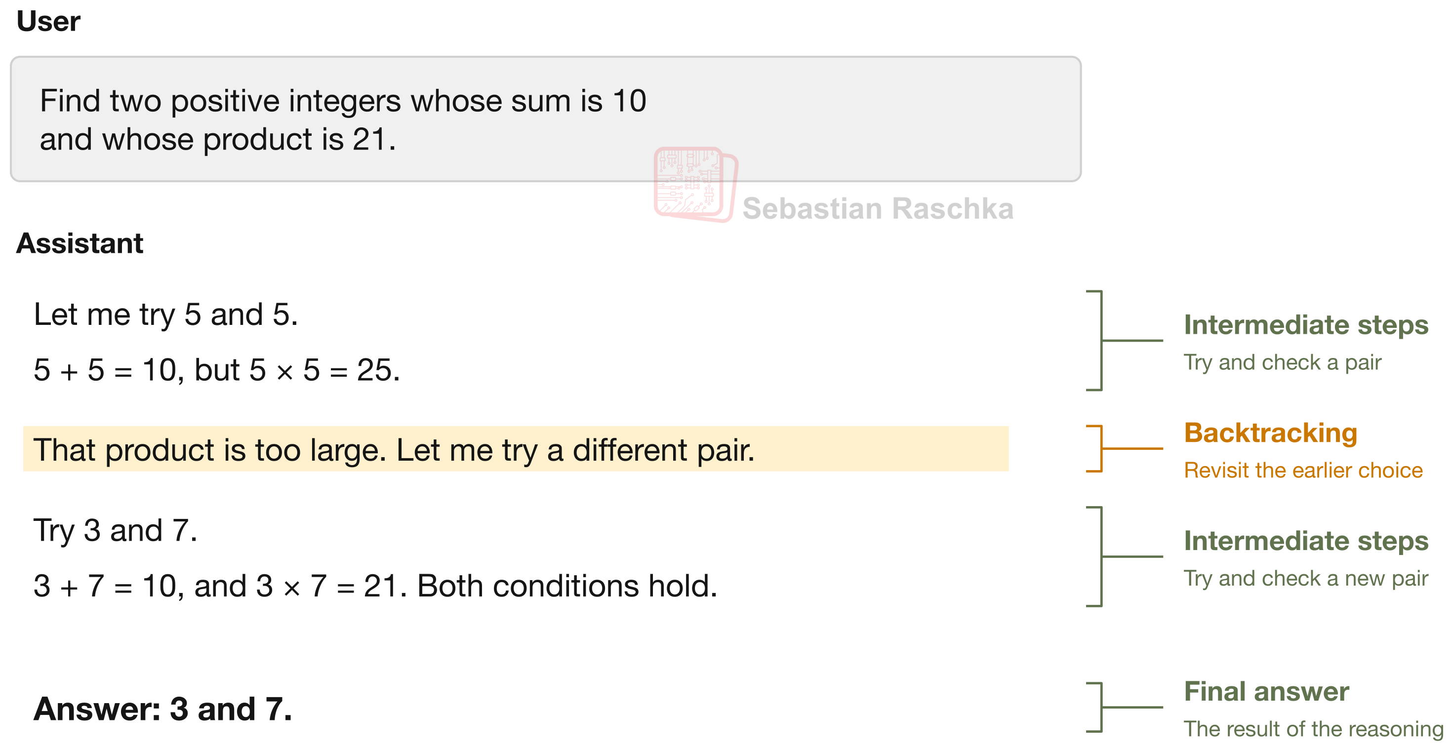
该图展示了推理模型如何“推理”，包括回溯。也就是说，模型发现了一个错误，然后重新审视之前的选择，再以不同的方法继续。

请注意，模型仍然是一次生成一个 token，并使用提示词和之前的 token 作为上下文。因此，这些中间步骤起到了草稿纸的作用，在最终答案之前增加了计算量。

如上例所示，最终答案可以比其之前的推理轨迹短得多。（OpenAI 倾向于向用户隐藏大部分推理轨迹。）

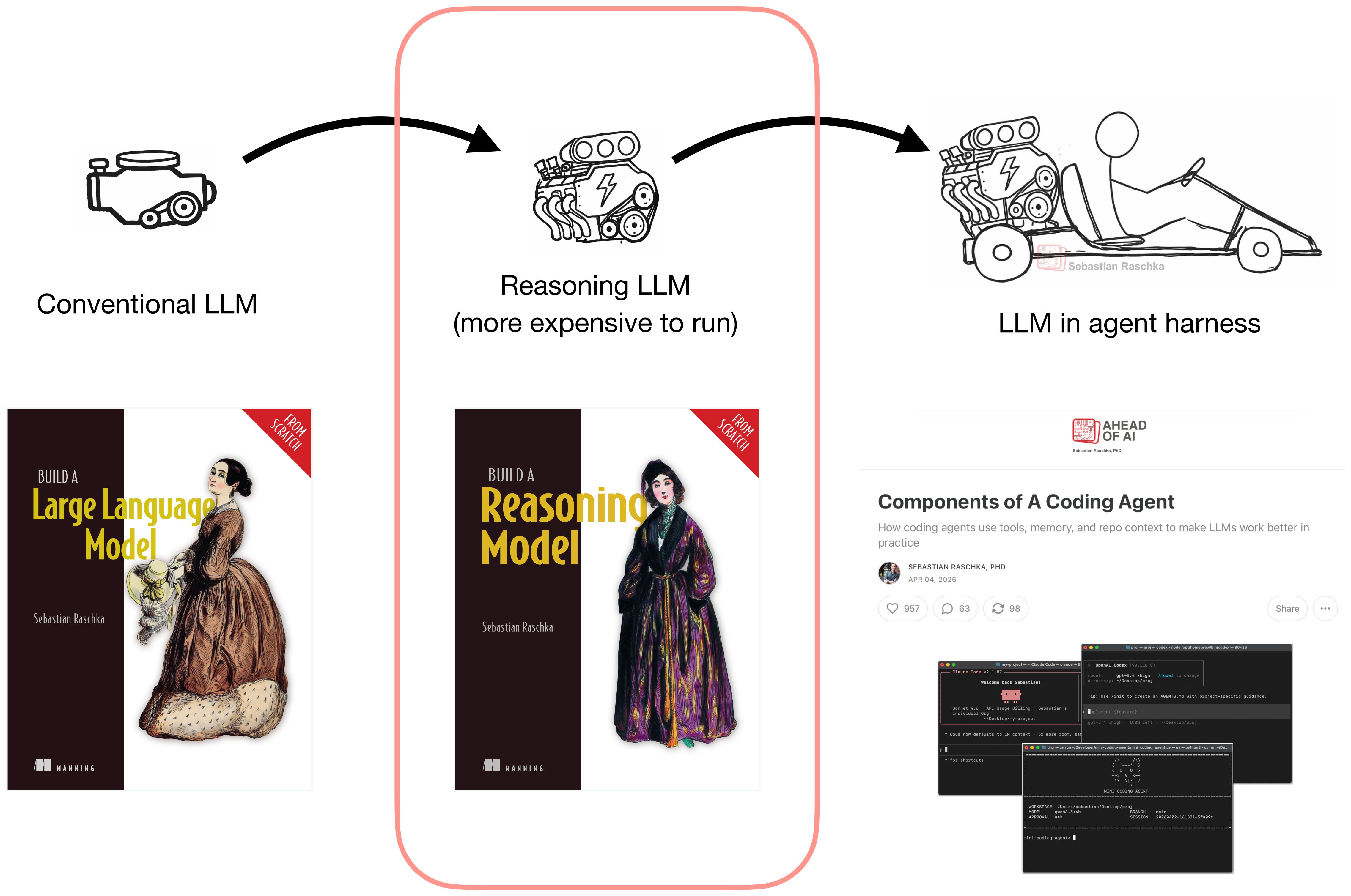
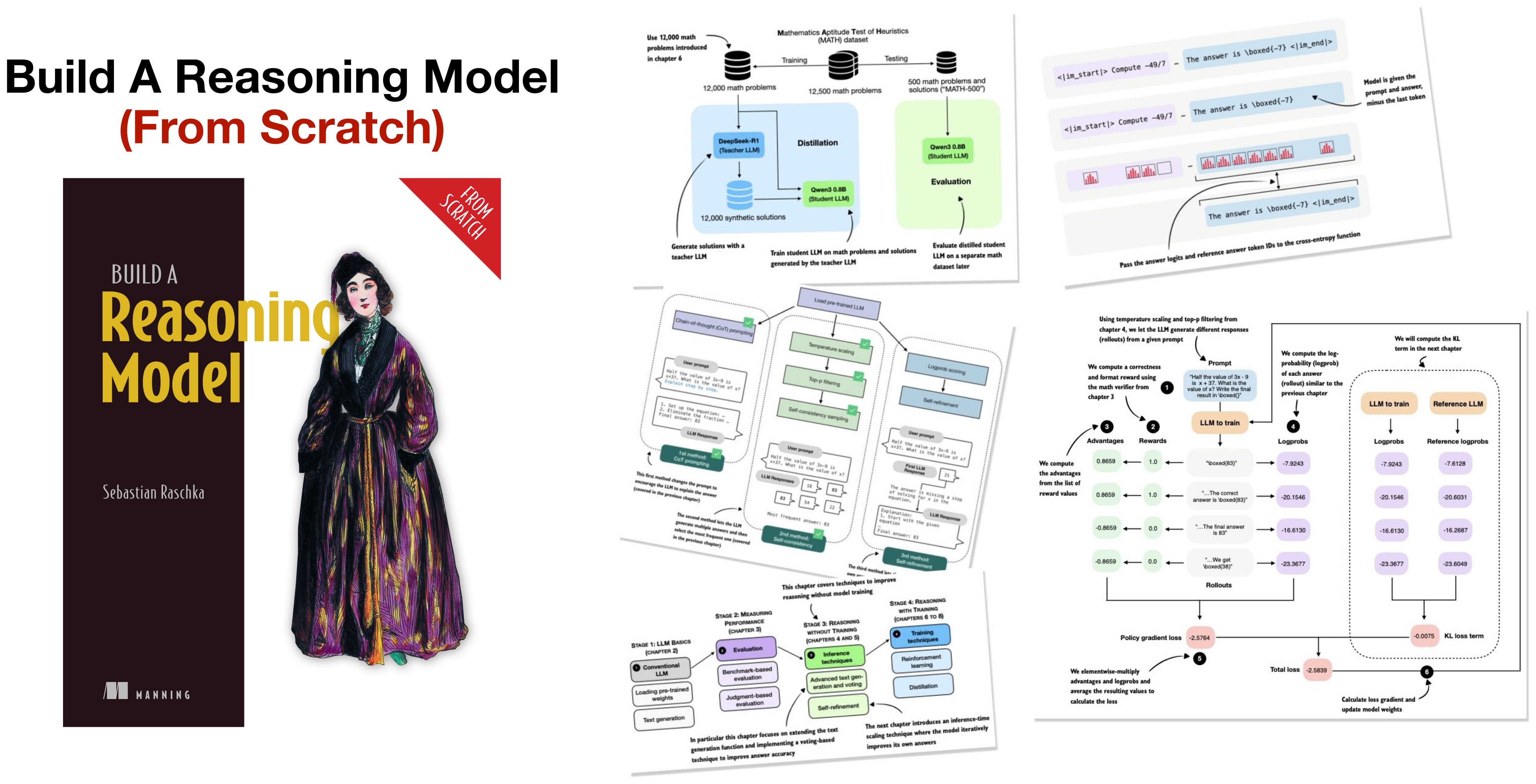
关于理解和开发推理模型的更多细节，我推荐我的书 《从零构建推理模型》。

5.2 Token 使用量与更短的思维链

现在，推理轨迹中额外的 token 会增加计算量。循环 Transformer 架构也会增加计算量，因为 token 会经过更多 Transformer 模块。有人可能会说，采用循环结构的模型在内部使用了更多计算，因此不需要那么多外部思考 token。

下面选取了 GPT-6 基准测试 的部分结果，横轴为输出 token 数量。

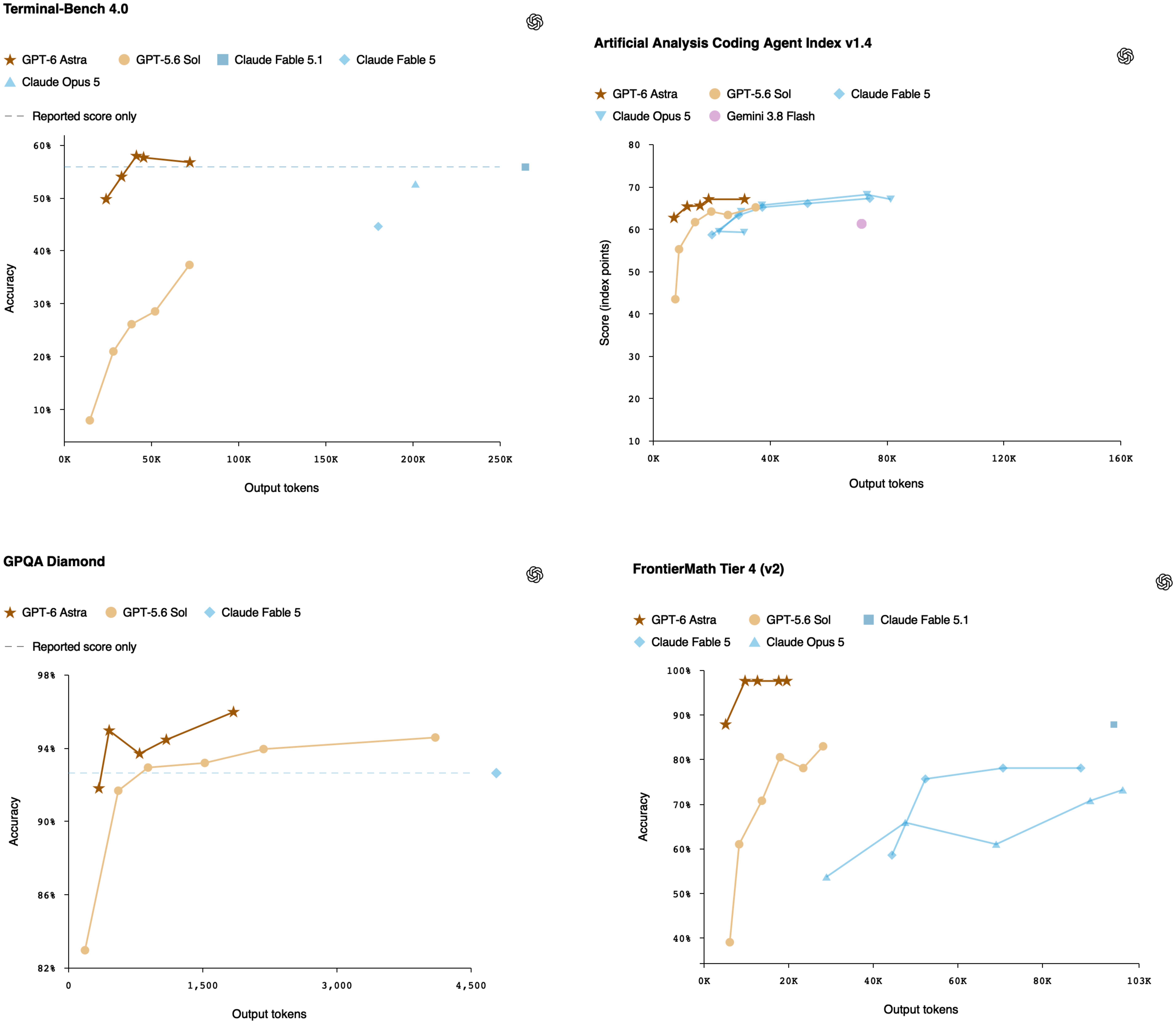
我们可以看到，在各个努力水平上，GPT-6 Astra 整体上并不一定比其前代 GPT 5.6 Sol 使用更少的 token。不过，在固定准确率下，GPT-6 Astra 确实比 GPT 5.6 Sol 使用更少的 token。

这是否会引发可解释性方面的担忧？未必。使用更少的 token 可能仅仅意味着模型能力更强、犯的错误更少、回溯更少等等。也就是说，它可能只是更常在第一次尝试时就做对。在我看来，这并不会立刻引发可解释性方面的担忧。

我的意思是，之前的模型也是如此。我不认为有人会强烈担忧 GPT 5.6 Sol 比更小的 GPT 5.6 Luna 模型可解释性差很多——后者在完成相同任务表现时需要更多 token，如下所示。

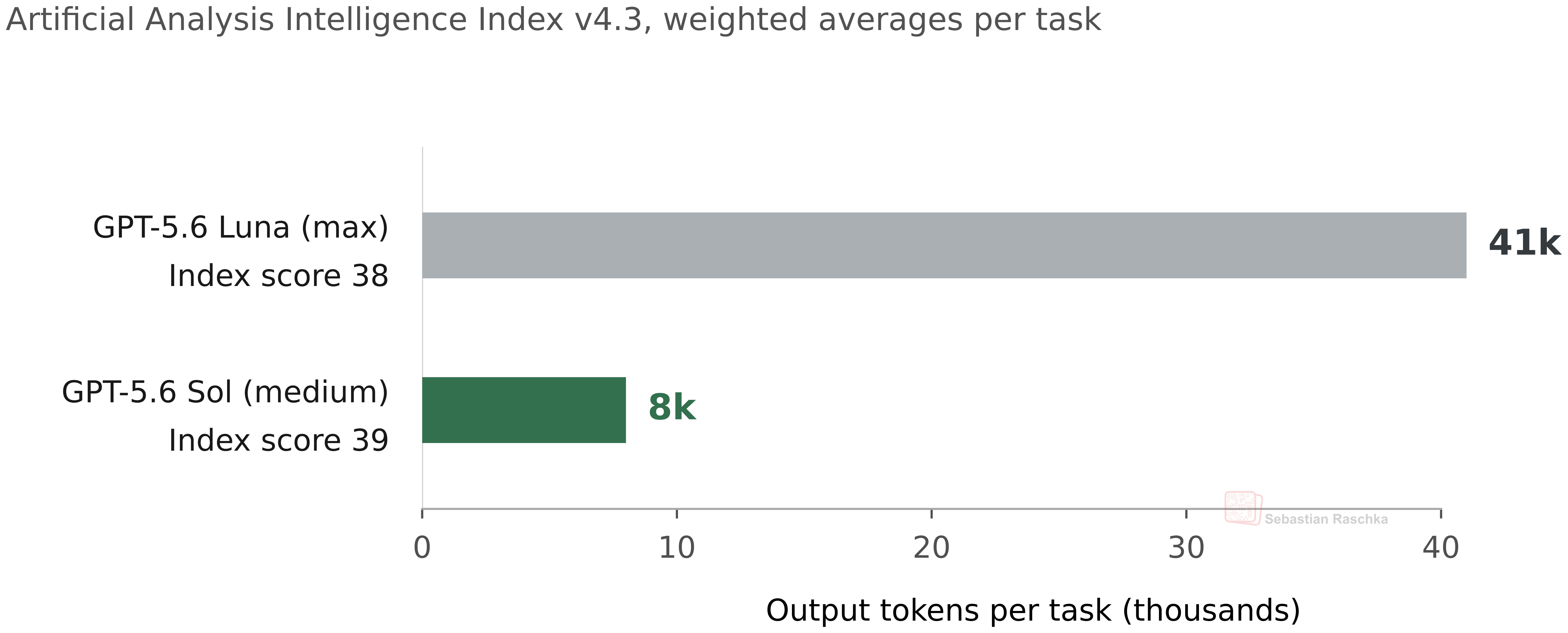
事实上，我们可以看到，在相近的建模性能下，Luna 消耗的模型 token 比 Sol 多 80%。这是否意味着 Sol 的可解释性就差那么多？

更合理的解释其实是：能力更强的模型（更大、训练充分、消耗更多算力的模型）能更高效地解决问题，这里的“高效”指的是消耗更少的模型 token。

同样值得记住的是，推理轨迹并不能保证忠实描述模型内部发生的一切。在我看来，唯一合理的担忧是，循环 Transformer 比传统 Transformer 更常刻意通过呈现“伪造”的推理轨迹来误导用户。但我认为我们还没有强有力的证据表明这种情况正在发生。

现在，Astra 的系统卡确实表明，有证据显示其推理轨迹的可监控性有所下降，并且相对于 Sol 存在一定程度的性能回退。这主要与更短、信息量更少的轨迹有关。但同样，这并不能证明循环是根本原因。这可能仅仅是因为轨迹整体较短所致，类似于上面 Luna 与 Sol 的例子。

在我分享关于循环 Transformer 可能隐藏推理链的看法几个小时后，Jakub Pachocki（OpenAI 首席科学家）也分享了以下澄清说明：

我想阻止一场由混乱报道引发的、滑向“无法监控”状态的竞赛。我们当前前沿模型（包括 Astra）的计算图深度，与 GPT-4 相差在两倍以内。OpenAI 从我们最早的推理模型起，就一直致力于保留并运用思维链监控技术。我们非常重视这项技术，因为它能让我们看到模型对齐如何从其训练分布中泛化出来。我确实认为这项技术是脆弱的，而且不幸的是它正朝着消极的方向发展，原因与架构变化无关，我很快会撰文详述。但我们可以采取一些措施来强化它，这也是我们当前研究计划的核心目标之一。

这里提到的“混乱报道”很可能指的是 The Information 上述段落，暗示循环这一方面与思维链的变化无关。

6. 循环 Transformer 架构研究

最后，我想分享一些与循环 Transformer 架构相关的有趣论文，这些论文超出了我们之前讨论的范围。

6.1 潜在推理

与 Universal Transformer 相关，2025 年的论文 《Scaling up Test-Time Compute with Latent Reasoning: A Recurrent Depth Approach》 研究了模型如何在推理时利用额外的循环。为此，他们在一个相对适中但也并非极小的 3.5B 参数模型上，用 800B tokens 进行了训练。

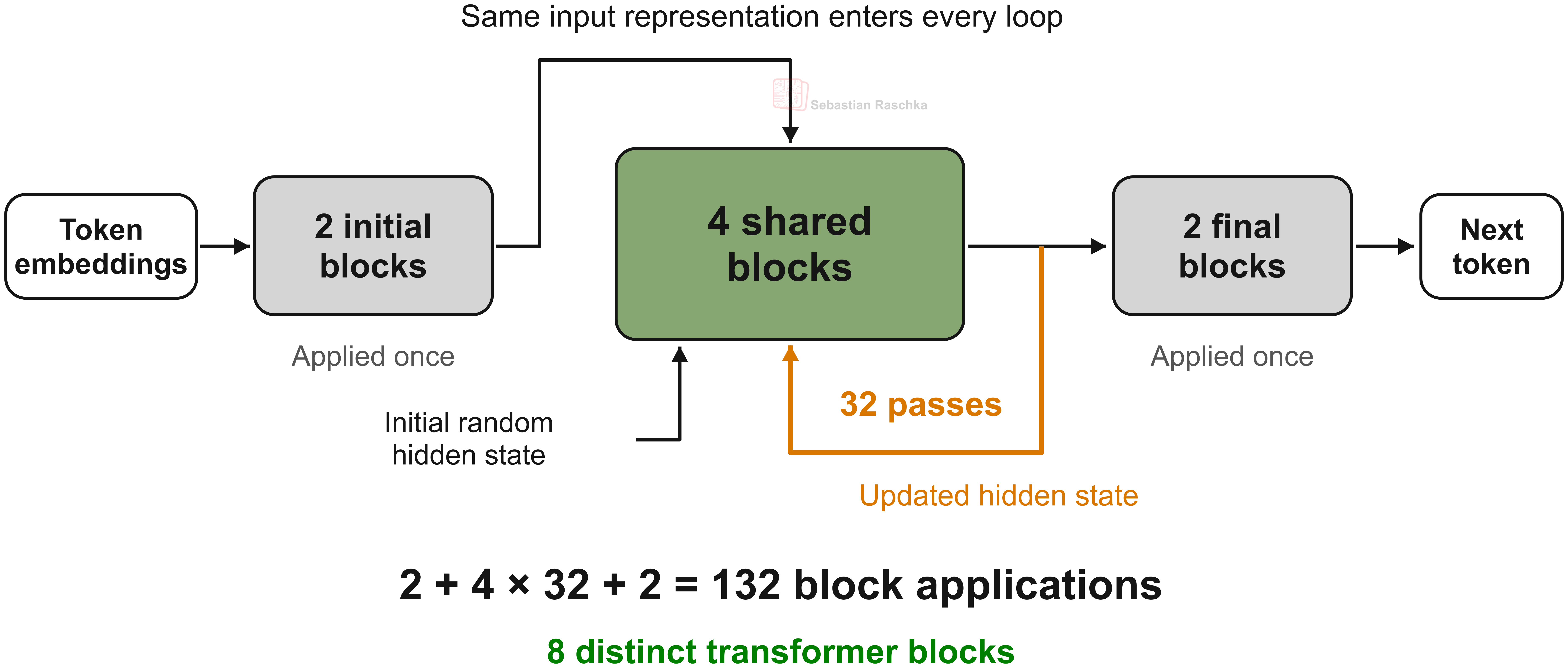
与 Universal Transformer 中反复复用同一个模块不同，它像 Nanbeige 那样重复一个堆叠结构；但与 Nanbeige 不同的是，它把这个共享的四模块堆叠夹在 2 个初始模块和 2 个最终模块之间。

此外，与 Nanbeige 的另一个区别是：在每一轮循环开始时，共享堆叠除了接收上一轮的隐藏状态之外，还会接收初始模块的输出。这两部分会被拼接起来，经过一个可学习的线性投影后再进入四个共享模块。你可以把这理解为：每次循环时，该堆叠都能访问到相同的初始输入表示。整个布局总结在下图中。

简而言之，这是一个额外的、有趣的循环 Transformer 变体。

一个有趣的细节是，研究人员在训练过程中会改变循环次数。这让模型能够适应推理时不同的计算量。

在这里，训练期间循环次数是随机采样的。推理时，由运行模型的人选择一个固定的预算，例如 8、32 或 64 次循环。此外，他们还针对每个 token 设计了一种基于下一个 token 概率分布的自适应停止机制。如果连续两轮之间的 KL 散度低于某个阈值——也就是说，如果两个分布过于相似——循环就会停止。

整体收益取决于具体任务。在他们的评估中，HellaSwag 的性能在大约八次循环后基本趋于平稳，而 GSM8K 和 HumanEval 则从更多循环中获益。

然而，尽管论文标题提到了“潜在推理”（latent reasoning），该模型仍然可以生成文本形式的思维链。循环只是在每个输出 token 之前为其提供额外的计算量。

6.2 知识检索与推理

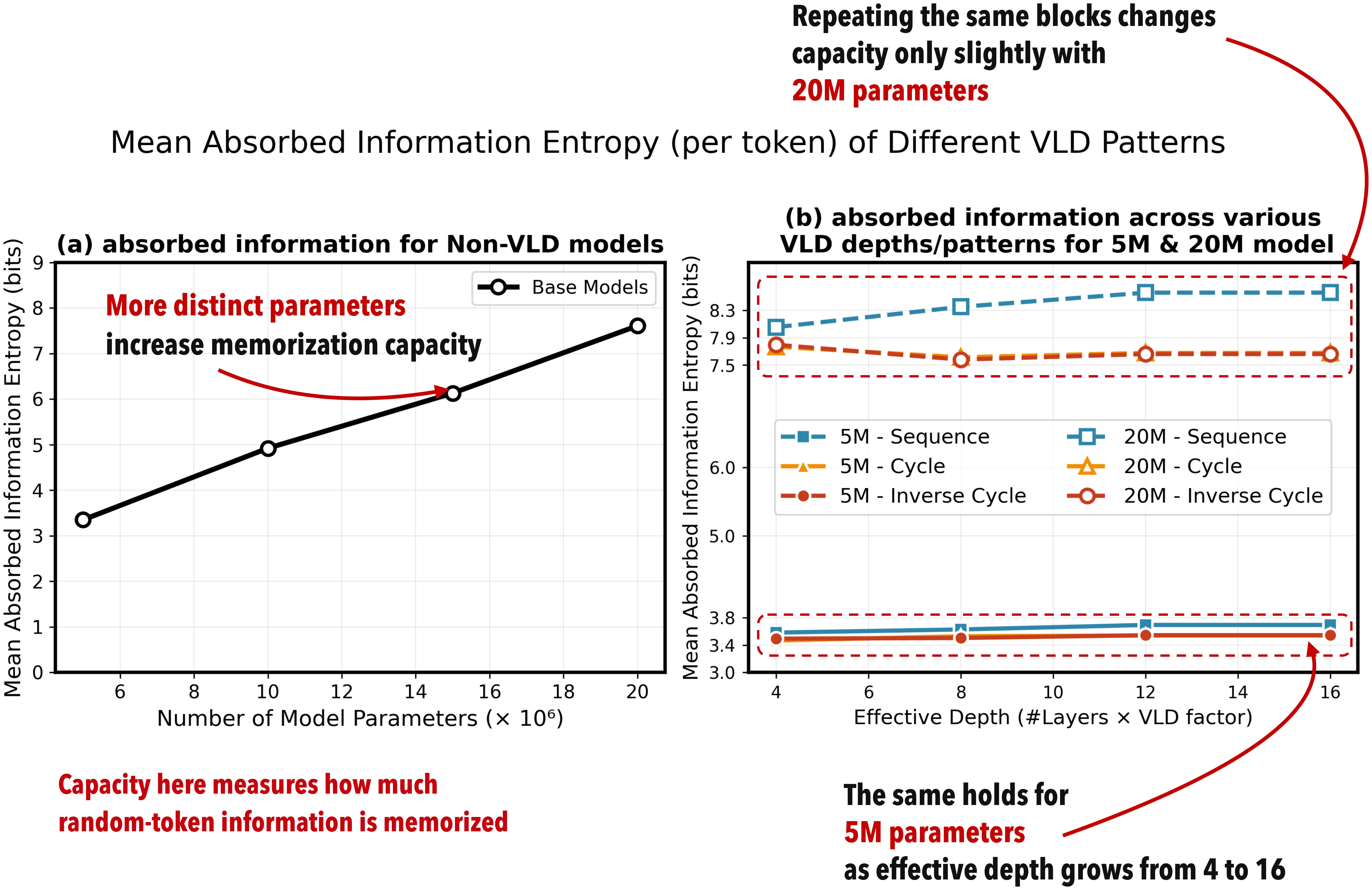
存储信息与使用信息来解决问题之间有一个有用的区分。例如，2025 年 6 月的论文 Beyond Parameters: Exploring Virtual Logic Depth for Scaling Laws 通过分别测量 LLM 中的记忆和推理来研究这一点。

首先，在记忆实验中，当参数数量保持不变时，循环几乎不会改变存储信息的数量。增加不同参数的数量确实会提升这种容量。由此我们可以得出结论：循环并不会增加模型可检索的知识，也不能让模型检索到更多知识。这是合理的。一旦信息被存储，信息检索就是一个相对简单的任务。此外，循环本身是一种计算机制，而非“存储”机制。

其次，在独立的推理实验中，在不增加参数的情况下，重用这些模块提升了多步数学问题的性能。这很有趣。在这里，我们可以得出结论：额外的计算可以帮助模型解决问题，即使它没有更多空间来存储信息。但同样，更大的模型也能提升推理能力（尽管它们同时也增加了参数）。

6.3 在匹配的计算预算下进行循环

刚刚发布的 SMELT：计算匹配的 MoE 循环 Transformer 的扩展定律 论文（2026 年 9 月）重新回到了第 2.2 节的成本比较。如果我们比较每 token 计算量、总非嵌入参数和 KV cache 需求大致相同的循环 Transformer 与传统 Transformer，会发生什么？

研究人员采用了混合专家（MoE）架构，并将 Transformer 模块的中间一半应用两次，这与 Nanbeige 的做法有些类似，只不过 Nanbeige 是在 Latent Reasoning 中采用了夹层结构。

然而，他们缩小了隐藏维度，以补偿额外模块应用所需的计算量。然后，由于这导致参数数量减少，他们又增加了专家数量以恢复总参数数量。他们还调整了注意力头配置，以保持 KV cache 的可比性。

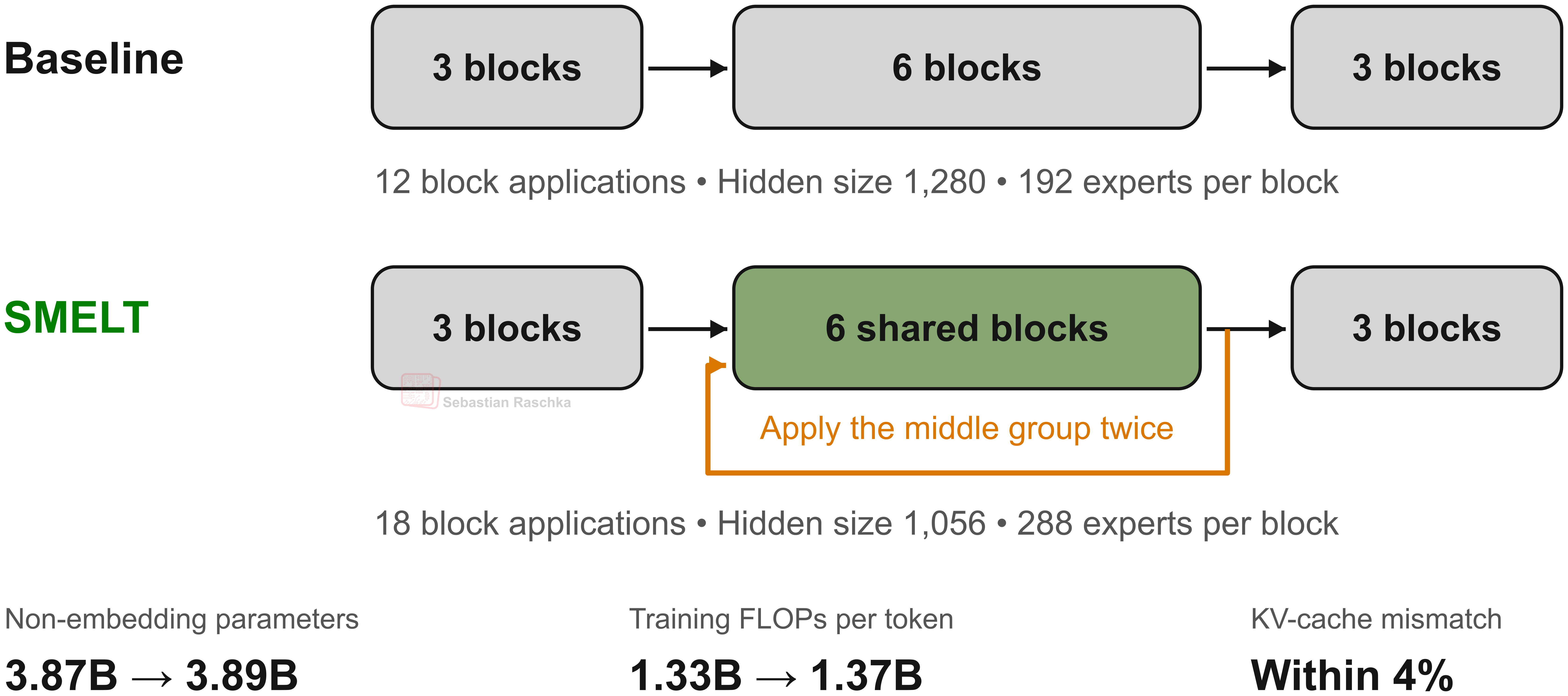
实验规模最高扩展到 54B 非嵌入参数等。然后，根据拟合的扩展曲线，研究人员估计，在所研究的计算量范围内，SMELT 达到相同验证损失所需的训练计算量大约减少 6.8-18%。

所以，这回答了循环 Transformer 在计算上是否值得的问题：是的！在相同的计算预算下，它们能给我们带来略好的模型。

6.4 全带宽 Transformer

最后，同样非常新的 全带宽 Transformer 论文（2026 年 8 月）研究了跨 token 位置的循环。在每一步解码时，它通过一个学习得到的门控，将前一个 token 的最终隐藏状态与新采样 token 的嵌入向量结合起来。这成为下一次前向传播的输入。

因此，下一个 token 的计算可以访问前一个 token 在堆栈底部的最终表示，这与潜在推理有些相似。

在使用 1B 基础模型时，他们发现其潜在反馈方法在 MATH500 上生成了更短的推理轨迹，同时保持或提高了准确率。然而，这种缩短效果在指令微调后消失了。

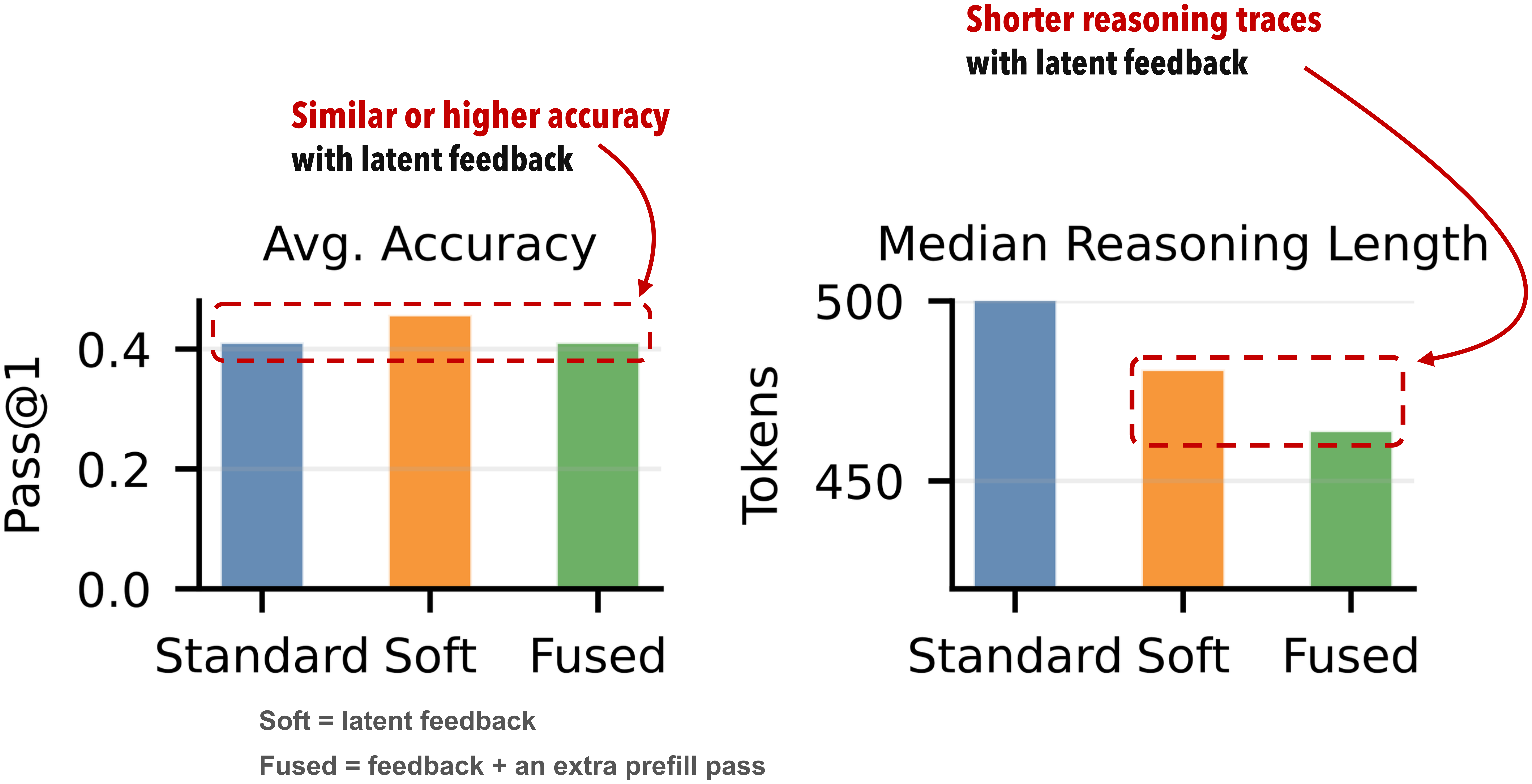
总之，这很有意思，因为它直接关联到前面关于循环是否会导致更短的推理轨迹的讨论。当然，结果既取决于反馈机制，也取决于模型的训练方式。此外，该实验并未证实那些更短的轨迹是否忠实度更低。

另外，这项研究的一个重大局限是，他们没有测试以传统方式增大模型规模（增加更多 Transformer 块而非循环）是否会对推理轨迹长度产生类似影响。

结论

总而言之，我们可以说，OpenAI GPT-6 Astra 确实是一个非常强大的模型。而且它在计算机使用方面取得了特别大的飞跃。我相信，在接下来的几个月里，计算机使用将成为开源和专有 harness 框架的下一个重点领域。我认为在计算机使用方面，开源尤其重要，因为“能力越大，责任越大”，在让它访问我的主电脑之前，能够审查 harness 框架是件好事。

此外，GPT-6 Astra 很可能使用了循环 Transformer 的一种变体。在固定的计算预算下，循环 Transformer 本身就提供了更好的建模性能。

而且，更好的建模性能可能会在更短的推理链中有所下降。但这并非新趋势。我们一直都能看到，在同一个模型家族中，不同规模的模型（例如 GPT 5.6 Luna 与 Sol）之间就存在这种情况。

在我看来，更短的推理轨迹是模型更“智能”或能力更强的副产品——这类模型犯错更少，并且能在其架构内部调用更多算力，而不必把推理轨迹当作草稿纸来用。从某种意义上说，人类也是如此。在大学的线下数学考试中，一个聪明且准备充分的学生可能不太需要用到草稿纸，需要回退重来的次数也更少，诸如此类。

感谢你阅读并支持我的工作！

如果你想学习如何自己构建推理模型，可以看看我的书 《从零构建推理模型》。我们从预训练的大语言模型出发，一步步为其加入推理能力，并附上你可以运行和实验的代码。这个过程既有趣又有收获，也是一笔对未来的自己很好的投资，帮你打好跟上 AI 领域发展的基本功。

另外，如果你读过我的书，我非常感激你能在 Amazon 上留下一段简短、真实的评价。评价能帮助其他读者判断一本书是否适合自己，也是支持作者的一种简单方式。